The Multiplicative Extended Kalman Filter

The MEKF is an important modification of the Kalman Filter that makes it applicable to orientation estimation. Unfortunately, when trying to research the topic for multirotor state estimation, I wasn’t able to find a simple (or recent!) explanation. This is my attempt to provide that simple summary.

You can see a short clip of it in action on a Beagle Bone Black with a MPU-9250 IMU here:

Setting the scene

Let’s imagine that you’re trying to write a multirotor control system to stabilise the craft in midair. Or maybe you’re writing software for your VR system of choice and need to estimate the pose of a handheld controller. Or perhaps you’re writing software that will switch a phone’s display between landscape and portrait mode depending on the detected orientation of the phone. In all of these cases, the device will have at least one onboard IMU (with at least a gyroscope and accelerometer and optionally, a magnetometer), and you’ll have to use the measurements from the IMU to derive an accurate estimate of the device orientation in 3D space. Unfortunately, the gyroscope and the accelerometer will be MEMS devices for the majority of consumer-grade hardware, which means they’ll be pretty noisy. Luckily, the devices provide redundant information, which we can use to dramatically improve any single-device dead-reckoning measurement. To do this we’ll need some ideas a few engineers at NASA came up with in the 60s.

You’ve probably also guessed that the Kalman filter is going to help here. Let’s think about that approach for a little bit. For the rest of the post, we’ll use the Hamiltonian convention for quaternions, and use $ R_b^i $ to refer to the rotation that converts from the body frame to the world frame, so that $ R_b^i v^b = v^i $. $ R_i^b $ will refer to the world-frame to body transformation, so $ R_i^b = {R_b^i}^T $. We want the orientation, so our state vector $ \boldsymbol{x} $ is going to at least partially be formed by an orientation parameterisation. For this thought experiment, we’re going to assume that we’re using a quaternion parameterisation, and that our state vector is formed only from the parameterisation, $ \boldsymbol{x} = q $ (for simplicity’s sake). Let’s assume we have our process and observation models worked out (or some equivalent linearisations) and have followed the usual Kalman filter update steps to get to the a posteriori state correction: $ \boldsymbol{x_{k|k}} = \boldsymbol{x_{k|k-1}} + K_k \boldsymbol{y_k} $. What kind of object is $ \boldsymbol{x_{k|k}} $? Well, $ \boldsymbol{x} $ is a unit quaternion, and we’re adding a non-zero value to it, so $ \boldsymbol{x_k} + K_k \boldsymbol{y_k} $ can’t be unitary. And if it’s not unitary, it can’t be a rotation. Kalman breaks one of the invariant properties of rotations that we need.

What happened? Well, we’ve fallen victim to one of the classic blunders: never assume that your operands are vectors! Rotation quaternions are not vectors. Neither are Euler angles (however you want to arrange them. No, really, they aren’t vectors), nor are rotation matrices. They are groups. And groups are not valid Kalman filter states, because they are only closed under their respective group operations, not under vector addition.

“Let’s not just throw the baby out with the bathwater just yet”, you argue. “We can recover from this. Just renormalise the sum.” And this can work (see, Multiplicative vs. Additive Filtering for Spacecraft Attitude Determination by Markeley, for example). But it throws off our a posteriori error correction, and what does the error covariance $P_{k|k} = cov(\boldsymbol{x} - \boldsymbol{\hat{x_{k|k}}})$ even mean now? We can slog through the math, but it gets pretty hairy, and there’s just something inelegant about plugging leaks like this. Let’s try a different approach.

Luckily, NASA solved this in the 60s by coming up with the MEKF. The trick is that we are going to assume that our orientation estimation is no longer captured by a single entry in the state vector. Instead, the full orientation representation $q$ (we’re still going to use quaternions) is captured by two parameters: an accumulated orientation estimate $ \hat{q} $, and separate small-angle error vector $ \boldsymbol{\alpha} $, which is used to parameterise an error quaternion, $\delta q(\boldsymbol{\alpha}) = \begin{pmatrix} 1 \\ \frac{\boldsymbol{\alpha}}{2} \end{pmatrix}$ , so our complete estimate is $ q = \hat{q} \delta q(\boldsymbol{\alpha}) $. Note the difference of this error operation compared to the naive error correction: because we have formulated the error in terms of the group operation, we maintain the invariance of this rotation representation.

Every filter update, the full-state estimate $ \hat{q} $ is first updated according to the measured angular velocity, $\boldsymbol{\hat{\omega}}$. Then, the small angle error is updated according to a standard Kalman filtering implementation (this works now, because $ \boldsymbol{\alpha} $ is guaranteed to be small, so we won’t run into any singularity issues). Finally, we update the full-state estimate with the error $ q_k = q_{k-1} \delta q_{k} $ and reset the quaternion small-angle error to unity: $\boldsymbol{\alpha_{k+1}} = \boldsymbol{0}$ and $\delta q_{k+1} = \begin{pmatrix} 1 \\ 0 \end{pmatrix}$

Multiplicative Extended Kalman Filter

So, the full steps (remembering that the state vector is initially $\boldsymbol{0}$) are:

First, update the orientation estimate with the measured angular velocity (this is unique to the MEKF):

$q_{k|k-1} = q_{k-1|k-1} + \dot{q}_{k-1|k-1} \Delta t = q_{k-1|k-1} + \frac{1}{2}q_{k-1|k-1} \begin{pmatrix} 0 \\ \boldsymbol{\omega} \end{pmatrix} \Delta t$

Then, update the process model:

$\Phi_k = (I + F\Delta t)$

where $ \dot{\boldsymbol{x}} = F \boldsymbol{x} $

Then, update the a priori estimate covariance and kalman gain (the following is common with the vanilla KF) :

$P_{k|k-1} = \Phi_k P_{k-1|k-1} \Phi_k^T + Q_k$ $K_k = P_{k|k-1} H_k^T (H_k P_{k|k-1} H_k^T + R_k)^{-1}$

Next, update the a posteriori state estimate and covariance:

$\boldsymbol{x_{k|k}} = K_k(\boldsymbol{z_k} - R_i^b(q_{k|k-1})\boldsymbol{f}^g)$ $P_{k|k} = (I - K_k H_k)P_{k|k-1}$

Finally, update the a posteriori orientation estimate (again, unique to the MEKF):

$q_{k|k} = q_{k|k-1} \delta q(x_{k|k})$

Concrete example with a gyroscope and accelerometer

Let’s work through a concrete implementation, where we have a single observation, an accelerometer measurement.

We assume the standard guassian noise with drift model for the gyroscope and accelerometer, so the measured angular velocity is the sum of the true angular velocity $ \boldsymbol{\omega} $, the bias $ \boldsymbol{\beta_{\omega}} $ and the white noise $ \boldsymbol{\eta_{\omega}} $: $ \boldsymbol{\hat{\omega}} = \boldsymbol{\omega} + \boldsymbol{\beta_{\omega}} + \boldsymbol{\eta_{\omega}} $. The bias drifts according to $ \dot{\boldsymbol{\beta_{\omega}}} = \boldsymbol{\nu_{\beta}} $ where $ \boldsymbol{\eta} $ and $ \boldsymbol{\nu} $ are white noise random processes.

Similarly, the accelerometer measures $ \boldsymbol{\hat{f}} = \boldsymbol{f} + \boldsymbol{\beta_{f}} + \boldsymbol{\eta_{f}} $ with drifting bias $ \beta_f $ and white noise $ \eta_f $. The true accelerometer measurement will be the sum of the acceleration from body-frame inertial forces $ \boldsymbol{f}^b $ and acceleration from gravity: $\boldsymbol{f}^b = \boldsymbol{a}^b + R(q)_i^b \begin{pmatrix} 0 \\ 0 \\ -g \end{pmatrix}^i$

Let’s form our state vector. We’ll need the orientation error parameterisation($\boldsymbol{\alpha}$), the position error ($\delta \boldsymbol{r}$) and linear velocity error ($\delta \boldsymbol{v}$) in world coordinates, and the gyro and accelerometer biases ($ \boldsymbol{\beta_{\omega}} $ and $ \boldsymbol{\beta_{f}}$):

$\boldsymbol{x} = \begin{pmatrix} \boldsymbol{\alpha} \\ \delta \boldsymbol{v} \\ \delta \boldsymbol{r} \\ \boldsymbol{\beta_{\omega}} \\ \boldsymbol{\beta_{f}} \end{pmatrix}$

In order to form the Kalman filter, we need to form our discrete state transition model, which is determined in the obvious form from the dynamics of the error state vector: $ \Phi = I + F\Delta t $ where $\dot{\boldsymbol{x}} = F \boldsymbol{x}$

See the appendix for derivations of the following.

$\dot{\boldsymbol{\alpha}} = -[\boldsymbol{\hat{\omega}} \times] \boldsymbol{\alpha} - \boldsymbol{\beta_{\omega}} - \boldsymbol{\eta_{\omega}}$ $\delta \dot{\boldsymbol{v}} = -R_b^i (\hat{q})[\boldsymbol{\hat{f}}^b \times] \boldsymbol{\alpha} - R_b^i(\hat{q}) \boldsymbol{\beta_f} - R_b^i (\hat{q}) \boldsymbol{\eta_f}$ $\delta \dot{\boldsymbol{r}} = \delta \boldsymbol{v}$ $\dot{\boldsymbol{\beta_{\omega}}} = \boldsymbol{\nu_{\omega}}$ $\dot{\boldsymbol{\beta_{f}}} = \boldsymbol{\nu_{f}}$

so,

$F = \begin{pmatrix}-[\boldsymbol{\hat{\omega}} \times] & 0 & 0 & -I & 0 \\ -R_b^i (\hat{q})[\boldsymbol{\hat{f}}^b \times] & 0 & 0 & 0 & - R_b^i(\hat{q}) \\ 0 & I & 0 & 0 & 0 \\ 0 & 0 & 0 & 0 & 0 \\ 0 & 0 & 0 & 0 & 0 \end{pmatrix}$

and

$Q_k = \int_0^{\Delta t} e^{F(\Delta t-\tau)} Q_c e^{F^T(\Delta t-\tau)} d\tau$

where

$Q_c = \begin{pmatrix} diag(\sigma_{\omega}^2) & 0 & 0 & 0 & 0 \\ 0 & diag(\sigma_{f}^2) & 0 & 0 & 0 \\ 0 & 0 & 0 & 0 & 0 \\ 0 & 0 & 0 & diag(\sigma_{\beta_{\omega}}^2) & 0 \\ 0 & 0 & 0 & 0 & diag(\sigma_{\beta_{f}}^2) \end{pmatrix}$

We can linearise $F$ around $\hat{\omega} = \hat{f} = 0 $ and $ R_i^b(\hat{q}) = I $ to obtain:

$Q_k = \begin{pmatrix} \wedge(\sigma_{\omega}^2) \Delta t + \wedge(\sigma_{\beta_{\omega}}^2) \frac{\Delta t^3}{3} & 0 & 0 & -\wedge(\sigma_{\beta_{\omega}}^2) \frac{\Delta t^2}{2} & 0 \\ 0 & \wedge(\sigma_f^2) \Delta t + \wedge(\sigma_{\beta_{f}}^2) \frac{\Delta t^3}{3} & \wedge(\sigma_{\beta_{f}}^2) \frac{\Delta t^4}{8} + \wedge(\sigma_{f}^2) \frac{\Delta t^2}{2} & 0 & -\wedge(\sigma_{\beta_{f}}^2) \frac{\Delta t^2}{2} \\ 0 & \wedge(\sigma_f^2) \frac{\Delta t^2}{2} + \wedge(\sigma_{\beta_{f}}^2) \frac{\Delta t^4}{8} & \wedge(\sigma_{f}^2) \frac{\Delta t^3}{3} + \wedge(\sigma_{\beta_f}^2) \frac{\Delta t^5}{20} & 0 & -\wedge(\sigma_{\beta_{f}}^2) \frac{\Delta t^3}{6} \\ -\wedge(\sigma_{\beta_{\omega}}^2) \frac{\Delta t^2}{2} & 0 & 0 & \wedge(\sigma_{\beta_{\omega}}^2) \Delta t & 0 \\ 0 & -\wedge(\sigma_{\beta_f}^2) \frac{\Delta t^2}{2} & -\wedge(\sigma_{\beta_f}^2) \frac{\Delta t^3}{6} & 0 & \wedge(\sigma_{\beta_{f}}^2) \Delta t \end{pmatrix}$

where $\wedge(\boldsymbol{x}) = \begin{pmatrix} x_0 & 0 & 0 \\ 0 & x_1 & 0 \\ 0 & 0 & x_2 \end{pmatrix}$

For the accelerometer observation,

$\delta \boldsymbol{f}^b = - \boldsymbol{\alpha} \times R_i^b(\hat{q}) \begin{pmatrix} 0 \\ 0 \\ -g \end{pmatrix} + \boldsymbol{\beta_f} + \boldsymbol{\eta_f}$

so,

$H = \begin{pmatrix} \begin{bmatrix}R_i^b(\hat{q})\begin{pmatrix} 0 \\ 0 \\ -g \end{pmatrix} \times \end{bmatrix} & 0 & 0 & 0 & I\end{pmatrix}$

Code

Here’s the python equivalent (you can find the full code here). You’ll notice a few details that we didn’t mention in the above, such as subtracting the estimated biases from the measurements:

class Kalman:

    #state vector:
    # [0:3] orientation error
    # [3:6] velocity error
    # [6:9] position error
    # [9:12] gyro bias
    # [12:15] accelerometer bias
    def __init__(self, initial_est, estimate_covariance, 
                       gyro_cov, gyro_bias_cov, accel_proc_cov, 
                       accel_bias_cov, accel_obs_cov):
        self.estimate = initial_est
        self.estimate_covariance = estimate_covariance*np.identity(15, dtype=float)

        self.observation_covariance = accel_obs_cov*np.identity(3, dtype=float)
        self.gyro_bias = np.array([0.0, 0.0, 0.0])
        self.accelerometer_bias = np.array([0.0, 0.0, 0.0])

        self.G = np.zeros(shape=(15, 15), dtype=float)
        self.G[0:3, 9:12] = -np.identity(3)
        self.G[6:9, 3:6] =  np.identity(3)

        self.gyro_cov_mat = gyro_cov*np.identity(3, dtype=float)
        self.gyro_bias_cov_mat = gyro_bias_cov*np.identity(3, dtype=float)
        self.accel_cov_mat = accel_proc_cov*np.identity(3, dtype=float)
        self.accel_bias_cov_mat = accel_bias_cov*np.identity(3, dtype=float)

    def process_covariance(self, time_delta):
        Q = np.zeros(shape=(15, 15), dtype=float)
        Q[0:3, 0:3] = self.gyro_cov_mat*time_delta + self.gyro_bias_cov_mat*(time_delta**3)/3.0
        Q[0:3, 9:12] = -self.gyro_bias_cov_mat*(time_delta**2)/2.0
        Q[3:6, 3:6] = self.accel_cov_mat*time_delta + self.accel_bias_cov_mat*(time_delta**3)/3.0
        Q[3:6, 6:9] = self.accel_bias_cov_mat*(time_delta**4)/8.0 + self.accel_cov_mat*(time_delta**2)/2.0
        Q[3:6, 12:15] = -self.accel_bias_cov_mat*(time_delta**2)/2.0
        Q[6:9, 3:6] = self.accel_cov_mat*(time_delta**2)/2.0 + self.accel_bias_cov_mat*(time_delta**4)/8.0
        Q[6:9, 6:9] = self.accel_cov_mat*(time_delta**3)/3.0 + self.accel_bias_cov_mat*(time_delta**5)/20.0
        Q[6:9, 12:15] = -self.accel_bias_cov_mat*(time_delta**3)/6.0
        Q[9:12, 0:3] = -self.gyro_bias_cov_mat*(time_delta**2)/2.0
        Q[9:12, 9:12] = self.gyro_bias_cov_mat*time_delta
        Q[12:15, 3:6] = -self.accel_bias_cov_mat*(time_delta**2)/2.0
        Q[12:15, 6:9] = -self.accel_bias_cov_mat*(time_delta**3)/6.0
        Q[12:15, 12:15] = self.accel_bias_cov_mat*time_delta

        return Q
        
    def update(self, gyro_meas, acc_meas, time_delta):
        
        gyro_meas = gyro_meas - self.gyro_bias
        acc_meas = acc_meas - self.accelerometer_bias

        #Integrate angular velocity through forming quaternion derivative 
        self.estimate = self.estimate + time_delta*0.5*self.estimate*Quaternion(scalar = 0, vector=gyro_meas)
        self.estimate = self.estimate.normalised

        #Form process model
        self.G[0:3, 0:3] = -skewSymmetric(gyro_meas)
        self.G[3:6, 0:3] = -quatToMatrix(self.estimate).dot(skewSymmetric(acc_meas))
        self.G[3:6, 12:15] = -quatToMatrix(self.estimate)
        F = np.identity(15, dtype=float) + self.G*time_delta

        #Update with a priori covariance
        self.estimate_covariance = np.dot(np.dot(F, self.estimate_covariance), F.transpose()) + self.process_covariance(time_delta)

        #Form Kalman gain
        H = np.zeros(shape=(3,15), dtype=float)
        H[0:3, 0:3] = skewSymmetric(self.estimate.inverse.rotate(np.array([0.0, 0.0, -1.0])))
        H[0:3, 12:15] = np.identity(3, dtype=float)
        PH_T = np.dot(self.estimate_covariance, H.transpose())
        inn_cov = H.dot(PH_T) + self.observation_covariance
        K = np.dot(PH_T, np.linalg.inv(inn_cov))

        #Update with a posteriori covariance
        self.estimate_covariance = (np.identity(15) - np.dot(K, H)).dot(self.estimate_covariance)
        
        aposteriori_state = np.dot(K, (acc_meas - self.estimate.inverse.rotate(np.array([0.0, 0.0, -1.0]))))

        #Fold filtered error state back into full state estimates
        self.estimate = self.estimate * Quaternion(scalar = 1, vector = 0.5*aposteriori_state[0:3])
        self.estimate = self.estimate.normalised
        self.gyro_bias += aposteriori_state[9:12]
        self.accelerometer_bias += aposteriori_state[12:15]

Results

How does this perform? Let’s simulate an object that starts at rest with no rotation and then begins rotating according to some random angular velocity. In this way, the object will move randomly, but smoothly. We inject some bias and gaussian noise into the simulated gyro and accelerometer measurements as well. Here are the results, compared to a naive dead reckoning integration of the gyro measurements:

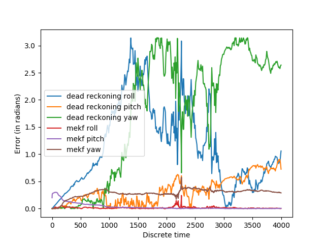
The roll and pitch are predicted accurately, but not yaw. This is expected: the accelerometer measures gravity, which is parallel to the yaw axis for the initial orientation. We can correct this by adding an additional reference measurement, such as from a magnetometer. We do this in the exact same way as the accelerometer, except the reference direction is now assumed to be $\begin{pmatrix} 1 \\ 0 \\ 0 \end{pmatrix}$ . The direction is not important as long as it is linearly independent of the body-frame z-axis.

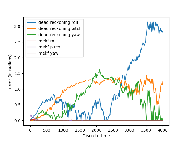
That’s better.

Appendix

The following derivations are from the excellent paper Multiplicative Quaternion Extended Kalman Filtering for Nonspinning Guided Projectiles by James M. Maley, with some corrections of mine for the derivations of the process covariance matrix.

Proof of $ \dot{\boldsymbol{\alpha}} = -[\boldsymbol{\hat{\omega}} \times] \boldsymbol{\alpha} - \boldsymbol{\beta_{\omega}} - \boldsymbol{\eta_{\omega}}$:

$\delta \dot{q} = \hat{q}^{-1} \dot{q} + \dot{\hat{q}}^{-1} q $

$\hat{q}^{-1} \hat{q} = 1$ , so $\frac{d(\hat{q}^{-1} \hat{q})}{dt} = 0$

Also, by the product rule: $\frac{d(\hat{q}^{-1} \hat{q})}{dt} = \dot{\hat{q}}^{-1} \hat{q} + \hat{q}^{-1} \dot{\hat{q}} $

So $\dot{\hat{q}}^{-1} = -\hat{q}^{-1} \dot{\hat{q}} \hat{q}^{-1}$ $= -\hat{q}^{-1} \frac{1}{2} \hat{q} \begin{pmatrix} 0 \\ \hat{\boldsymbol{\omega}}^b \end{pmatrix} \hat{q}^{-1}$ $= - \frac{1}{2}\begin{pmatrix} 0 \\ \hat{\boldsymbol{\omega}}^b \end{pmatrix}\hat{q}^{-1}$

Using this definition in $\delta \dot{q} = \hat{q}^{-1} \dot{q} + \dot{\hat{q}}^{-1} q $:

$\delta \dot{q} = \hat{q}^{-1} \frac{1}{2}q \begin{pmatrix} 0 \\ \boldsymbol{\omega}^b \end{pmatrix} - \frac{1}{2}\begin{pmatrix} 0 \\ \hat{\boldsymbol{\omega}}^b \end{pmatrix}\hat{q}^{-1} q$ $\delta \dot{q} = \frac{1}{2}\delta q \begin{pmatrix} 0 \\ \boldsymbol{\omega}^b \end{pmatrix} - \frac{1}{2}\begin{pmatrix} 0 \\ \hat{\boldsymbol{\omega}}^b \end{pmatrix}\delta q$ $\delta \dot{q} = \frac{1}{2}\delta q \begin{pmatrix} 0 \\ \hat{\boldsymbol{\omega}}^b \end{pmatrix} - \frac{1}{2}\begin{pmatrix} 0 \\ \hat{\boldsymbol{\omega}}^b \end{pmatrix}\delta q + \frac{1}{2}\delta q \begin{pmatrix} 0 \\ \delta \boldsymbol{\omega} \end{pmatrix}$

Using the definition of quaternion multiplication and $\delta q_r \approx 1$:

$\delta \dot{q} = \frac{1}{2} \begin{pmatrix} -\delta \boldsymbol{q_v} \cdot \hat{\boldsymbol{\omega}} \\ \hat{\boldsymbol{\omega}}^b + \delta \boldsymbol{q_v} \times \hat{\boldsymbol{\omega}} \end{pmatrix} + \frac{1}{2}\begin{pmatrix} \hat{\boldsymbol{\omega}} \cdot \delta \boldsymbol{q_v} \\ -\hat{\boldsymbol{\omega}}^b - \hat{\boldsymbol{\omega}} \times \delta \boldsymbol{q_v} \end{pmatrix} + \frac{1}{2}\begin{pmatrix} -\delta \boldsymbol{q_v} \cdot \delta \hat{\boldsymbol{\omega}} \\ \delta \hat{\boldsymbol{\omega}} + \delta \boldsymbol{q_v} \times \delta \hat{\boldsymbol{\omega}} \end{pmatrix}$

Simplying the vector component of this quaternion, and setting the second-order error components to $0$, we obtain:

$\delta \boldsymbol{q_v} = -\hat{\boldsymbol{\omega}} \times \delta \boldsymbol{q_v} + \frac{1}{2} \delta \boldsymbol{\omega}$

and using our definition of $\boldsymbol{\alpha}$, $\boldsymbol{\alpha} = 2\delta \boldsymbol{q_v}$, this becomes:

$\dot{\boldsymbol{\alpha}} = -[\boldsymbol{\hat{\omega}} \times] \boldsymbol{\alpha} + \delta \boldsymbol{\omega}$

which is the result we wanted.

Proof of $ \delta \boldsymbol{f}^b = - \boldsymbol{\alpha} \times R_i^b(\hat{q}) \boldsymbol{m}^i + \boldsymbol{\beta_f} + \boldsymbol{\eta_f} $:

The measured reference is going to be a function of the reference vector and the true orientation and measurement bias and noise:

$\boldsymbol{m} = R_i^b(q) \boldsymbol{m}^i + \boldsymbol{\beta_m} + \boldsymbol{\eta_m}$

The estimated observation is a function of the reference vector and current quaternion estimate:

$\hat{\boldsymbol{m}} = R_i^b(\hat{q}) \boldsymbol{m}^i$

We have the following equivalence (see Rodrigues’ rotation formula):

$R_i^b(q) = 2 \boldsymbol{q_v} \boldsymbol{q_v}^T + I_{3 \times 3}(q_r^2 - \boldsymbol{q_v}^T \boldsymbol{q_v}) - 2q_r[\boldsymbol{q_v} \times]$

so (ignoring second-order error terms):

$R_i^b(\delta q) = I - [\boldsymbol{\alpha} \times]$

and

$R_i^b(q) = R_i^b(\delta q) R_i^b(\hat{q}) = (I - [\boldsymbol{\alpha} \times])R_i^b(\hat{q})$

$\delta \boldsymbol{m}^b = \boldsymbol{m}^b - \hat{\boldsymbol{m}}^b = (I - [\boldsymbol{\alpha} \times])R_i^b(\hat{q}) \boldsymbol{m}^i + \boldsymbol{\beta_m} + \boldsymbol{\eta_m} - R_i^b(\hat{q}) \boldsymbol{m}^i$

$\delta \boldsymbol{m}^b = -[\boldsymbol{\alpha} \times])R_i^b(\hat{q}) \boldsymbol{m}^i + \boldsymbol{\beta_m} + \boldsymbol{\eta_m}$

which is the required result.

Proof of a priori covariance propagation

From earlier, we have:

Using the previous definitions of $ \boldsymbol{x} $ and $ F $, we can restate this as:

$\dot{\boldsymbol{x}} = F \boldsymbol{x} + G \boldsymbol{w}$

with

$G = \begin{pmatrix} diag(-\sigma_{\omega}) & 0 & 0 & 0 & 0 \\ 0 & -R_b^i(\hat{q}) diag(\sigma_f) & 0 & 0 & 0 \\ 0 & 0 & 0 & 0 & 0 \\ 0 & 0 & 0 & diag(\sigma_{\beta_{\omega}}) & 0 \\ 0 & 0 & 0 & 0 & diag(\sigma_{\beta_f})) \end{pmatrix}$

and $ \boldsymbol{w} $, a unity-variance, zero mean white-noise vector.

By inspection, the cross-correlation of $G\boldsymbol{w}$ is

$E[(G\boldsymbol{w}(t))(G\boldsymbol{w}(\tau))^T] = Q_c \delta(t - \tau)$

The solution of $ \dot{\boldsymbol{x}} = F \boldsymbol{x} + G \boldsymbol{w} $ is a well-known result:

$\boldsymbol{x}(t) = e^{F(t - t_0)}\boldsymbol{x}(t_0) + \int_{t_0}^{t} e^{F(t - \tau)} G\boldsymbol{w}(\tau) d\tau$

We are interested in $ t = t_k $ and $ t_0 = t_{k-1} $, so that $ t_k - t_{k-1} = \Delta t $, and make the substitution in the integral of $ \tau’ = \tau - t_{k-1} $

$\boldsymbol{x}(t_k) = e^{F\Delta t}\boldsymbol{x}(t_{k-1}) + \int_{0}^{\Delta t} e^{F(\Delta t - \tau')} G\boldsymbol{w}(\tau' + t_{k-1}) d\tau'$

The covariance of $ \boldsymbol{x}(t_k) $ is then given by:

$P_{k|k-1} = E[\boldsymbol{x}(t_k)\boldsymbol{x}(t_k)^T] = E[\begin{pmatrix} e^{F\Delta t}\boldsymbol{x}(t_{k-1}) + \int_{0}^{\Delta t} e^{F(\Delta t - \tau')} G\boldsymbol{w}(\tau' + t_{k-1}) d\tau' \end{pmatrix} \begin{pmatrix} e^{F\Delta t}\boldsymbol{x}(t_{k-1}) + \int_{0}^{\Delta t} e^{F(\Delta t - \tau'')} G\boldsymbol{w}(\tau'' + t_{k-1}) d\tau''\end{pmatrix}^T]$

Expanding this, we drop products of $ \boldsymbol{x} $ and $ \boldsymbol{w} $, because they are uncorrelated and both have an expectation of 0:

$E[\boldsymbol{x}(t_k)\boldsymbol{x}(t_k)^T] = e^{F\Delta t} E[\boldsymbol{x}(t_{k-1})\boldsymbol{x}(t_{k-1})^T] e^{F^T\Delta t} + \int_{0}^{\Delta t}\int_{0}^{\Delta t} e^{F(\Delta t - \tau')} E[G\boldsymbol{w}(\tau' + t_{k-1})\boldsymbol{w}(\tau'' + t_{k-1})^TG^T]e^{F^T(\Delta t - \tau'')} d\tau' d\tau''$ $E[\boldsymbol{x}(t_k)\boldsymbol{x}(t_k)^T] = e^{F\Delta t} P_{(k-1|k-1)} e^{F^T\Delta t} + \int_{0}^{\Delta t}\int_{0}^{\Delta t} e^{F(\Delta t - \tau')} Q_c \delta(\tau' - \tau'') e^{F^T(\Delta t - \tau'')} d\tau' d\tau''$ $E[\boldsymbol{x}(t_k)\boldsymbol{x}(t_k)^T] = \Phi P_{(k-1|k-1)} \Phi^T + \int_{0}^{\Delta t} e^{F(\Delta t - \tau'')} Q_c e^{F^T(\Delta t - \tau'')}d\tau''$

So, $Q_k = \int_{0}^{\Delta t} e^{F(\Delta t - \tau)} Q_c e^{F^T(\Delta t - \tau)}d\tau$, the desired result.

We approximate $ e^{F(\Delta t - \tau)} $ with $ I + F(\Delta t - \tau) + \frac{1}{2} F^2(\Delta t - \tau)^2 $ and linearise $F$ around $\hat{\omega} = \hat{f} = 0 $ and $ R_i^b(\hat{q}) = I $, so that

$F \approx \begin{pmatrix} 0 & 0 & 0 & -I & 0 & 0 \\ 0 & 0 & 0 & 0 & -I & 0 \\ 0 & I & 0 & 0 & 0 & 0 \\ 0 & 0 & 0 & 0 & 0 & 0 \\ 0 & 0 & 0 & 0 & 0 & 0 \\ 0 & 0 & 0 & 0 & 0 & 0 \end{pmatrix}$

and

$I + F(\Delta t - \tau) + \frac{1}{2} F^2(\Delta t - \tau)^2$ =

$\begin{pmatrix} I & 0 & 0 & -I(\Delta t - \tau) & 0 & 0 \\ 0 & I & 0 & 0 & -I(\Delta t - \tau) & 0 \\ 0 & I(\Delta t - \tau) & I & 0 & -\frac{I}{2}(\Delta t - \tau)^2 & 0 \\ 0 & 0 & 0 & I & 0 & 0 \\ 0 & 0 & 0 & 0 & I & 0 \\ 0 & 0 & 0 & 0 & 0 & I \end{pmatrix}$

Using this approximation in $e^{F(\Delta t - \tau)} Q_c e^{F^T(\Delta t - \tau)}$ gives us:

$Q_k = \int_{0}^{\Delta t} \begin{pmatrix} \wedge(\sigma_{\omega}^2) + \wedge(\sigma_{\beta_{\omega}}^2) (\Delta t - \tau)^2 & 0 & 0 & -\wedge(\sigma_{\beta_{\omega}}^2) (\Delta t - \tau) & 0 \\ 0 & \wedge(\sigma_f^2) + \wedge(\sigma_{\beta_{f}}^2) (\Delta t - \tau)^2 & \wedge(\sigma_{\beta_{f}}^2) \frac{(\Delta t - \tau)^3}{2} + \wedge(\sigma_{f}^2) (\Delta t - \tau) & 0 & -\wedge(\sigma_{\beta_{f}}^2)(\Delta t - \tau) \\ 0 & \wedge(\sigma_f^2) (\Delta t - \tau) + \wedge(\sigma_{\beta_{f}}^2) \frac{(\Delta t - \tau)^3}{2} & \wedge(\sigma_{f}^2)(\Delta t - \tau)^2 + \wedge(\sigma_{\beta_f}^2) \frac{(\Delta t - \tau)^4}{4} & 0 & -\wedge(\sigma_{\beta_{f}}^2) \frac{(\Delta t - \tau)^2}{2} \\ -\wedge(\sigma_{\beta_{\omega}}^2) (\Delta t - \tau) & 0 & 0 & \wedge(\sigma_{\beta_{\omega}}^2) & 0 \\ 0 & -\wedge(\sigma_{\beta_f}^2) (\Delta t - \tau) & -\wedge(\sigma_{\beta_f}^2) \frac{(\Delta t - \tau)^2}{2} & 0 & \wedge(\sigma_{\beta_{f}}^2) \end{pmatrix} d\tau$

Evaluating this integral gives us the desired result for the $Q_k$ process noise approximation.

Extended equations for a magnetometer observation

We extend our state vector to include the magnetometer bias:

$\boldsymbol{x} = \begin{pmatrix} \boldsymbol{\alpha} \\ \delta \boldsymbol{v} \\ \delta \boldsymbol{r} \\ \boldsymbol{\beta_{\omega}} \\ \boldsymbol{\beta_{f}} \\ \boldsymbol{\beta_m} \end{pmatrix}$

with $ \dot{\boldsymbol{\beta_m}} = \boldsymbol{\eta_{m}}$

Then $F$ becomes

$F = \begin{pmatrix}-[\boldsymbol{\hat{\omega}} \times] & 0 & 0 & -I & 0 & 0 \\ -R_b^i (\hat{q})[\boldsymbol{\hat{f}}^b \times] & 0 & 0 & 0 & - R_b^i(\hat{q}) & 0 \\ 0 & I & 0 & 0 & 0 & 0 \\ 0 & 0 & 0 & 0 & 0 & 0 \\ 0 & 0 & 0 & 0 & 0 & 0 \\ 0 & 0 & 0 & 0 & 0 & 0 \end{pmatrix}$

and $Q_c$ and $Q_k$ become

$Q_c = \begin{pmatrix} diag(\sigma_{\omega}^2) & 0 & 0 & 0 & 0 & 0 \\ 0 & diag(\sigma_{f}^2) & 0 & ) & 0 & 0 \\ 0 & 0 & 0 & 0 & 0 & 0 \\ 0 & 0 & 0 & diag(\sigma_{\beta_{\omega}}^2) & 0 & 0 \\ 0 & 0 & 0 & 0 & diag(\sigma_{\beta_{f}}^2) & 0 \\ 0 & 0 & 0 & 0 & 0 & diag(\sigma_{\beta_{m}}^2) \end{pmatrix}$ $Q_k = \begin{pmatrix} \wedge(\sigma_{\omega}^2) \Delta t + \wedge(\sigma_{\beta_{\omega}}^2) \frac{\Delta t^3}{3} & 0 & 0 & -\wedge(\sigma_{\beta_{\omega}}^2) \frac{\Delta t^2}{2} & 0 & 0 \\ 0 & \wedge(\sigma_f^2) \Delta t + \wedge(\sigma_{\beta_{f}}^2) \frac{\Delta t^3}{3} & \wedge(\sigma_{\beta_{f}}^2) \frac{\Delta t^4}{8} + \wedge(\sigma_{f}^2) \frac{\Delta t^2}{2} & 0 & -\wedge(\sigma_{\beta_{f}}^2) \frac{\Delta t^2}{2} & 0 \\ 0 & \wedge(\sigma_f^2) \frac{\Delta t^2}{2} + \wedge(\sigma_{\beta_{f}}^2) \frac{\Delta t^4}{8} & \wedge(\sigma_{f}^2) \frac{\Delta t^3}{3} + \wedge(\sigma_{\beta_f}^2) \frac{\Delta t^5}{20} & 0 & -\wedge(\sigma_{\beta_{f}}^2) \frac{\Delta t^3}{6} & 0 \\ -\wedge(\sigma_{\beta_{\omega}}^2) \frac{\Delta t^2}{2} & 0 & 0 & \wedge(\sigma_{\beta_{\omega}}^2) \Delta t & 0 & 0 \\ 0 & -\wedge(\sigma_{\beta_f}^2) \frac{\Delta t^2}{2} & -\wedge(\sigma_{\beta_f}^2) \frac{\Delta t^3}{6} & 0 & \wedge(\sigma_{\beta_{f}}^2) \Delta t & 0 \\ 0 & 0 & 0 & 0 & 0 & \wedge(\sigma_{\beta_m}^2) \Delta t \end{pmatrix}$

Similarly, the observation matrix $H$ becomes

$H = \begin{pmatrix} \begin{bmatrix}R_i^b(\hat{q})\begin{pmatrix} 0 \\ 0 \\ -g \end{pmatrix} \times \end{bmatrix} & 0 & 0 & 0 & I & 0 \\ \begin{bmatrix}R_i^b(\hat{q})\begin{pmatrix} 1 \\ 0 \\ 0 \end{pmatrix} \times \end{bmatrix} & 0 & 0 & 0 & 0 & I\end{pmatrix}$